Simulating publication bias

To see some effects of publication bias, let’s do a simulation.

Assume that there are five possible hypotheses and only one of them is actually true. Many studies will be done on each of the hypotheses.

run_study <- function (x, mu) {
  grp1 <- rnorm(x, mean = 0, sd = 3)
  grp2 <- rnorm(x, mean = 0 + mu, sd = 2)
  t.test(grp1, grp2)
}

p_val <- function (x, hyp) {
  if (hyp == 5) {
    return(run_study(x, mu = 1)$p.value)
  }
  run_study(x, mu = 0)$p.value
}

To start off, assume exactly 20 studies are done on each hypothesis.

set.seed(18)
res_hyp1 <- replicate(20, p_val(100, 1))
res_hyp2 <- replicate(20, p_val(100, 2))
res_hyp3 <- replicate(20, p_val(100, 3))
res_hyp4 <- replicate(20, p_val(100, 4))
res_hyp5 <- replicate(20, p_val(100, 5))

hyp1_effects <- sum(res_hyp1 < 0.05)
hyp2_effects <- sum(res_hyp2 < 0.05)
hyp3_effects <- sum(res_hyp3 < 0.05)
hyp4_effects <- sum(res_hyp4 < 0.05)
hyp5_effects <- sum(res_hyp5 < 0.05)

Let’s say we publish about 10% of the null results, and 75% of the non-null results:

published <- function() data.frame(
  hyp = 1:5,
  pub_eff = c(rbinom(1, hyp1_effects, p = .75),
              rbinom(1, hyp2_effects, p = .75),
              rbinom(1, hyp3_effects, p = .75),
              rbinom(1, hyp4_effects, p = .75),
              rbinom(1, hyp5_effects, p = .75)),
  pub_null = c(rbinom(1, 20 - hyp1_effects, p = .1),
               rbinom(1, 20 - hyp2_effects, p = .1),
               rbinom(1, 20 - hyp3_effects, p = .1),
               rbinom(1, 20 - hyp4_effects, p = .1),
               rbinom(1, 20 - hyp5_effects, p = .1))
)

set.seed(1957)
print(published())

##   hyp pub_eff pub_null
## 1   1       1        0
## 2   2       0        3
## 3   3       0        1
## 4   4       0        0
## 5   5      13        0

The first problem is that it isn’t clear from any individual study whether we have a true effect or not. But the bigger problem is that the literature is systematically biased away from the null. In fact, we sometimes have more non-null studies than null studies for a true null hypothesis:

any_unbalanced <- function () {
  result <- published()[1:4,]
  any(result$pub_eff > result$pub_null)
}

mean(replicate(1000, any_unbalanced()))

## [1] 0.221

So, under these assumptions, there is a 20% chance that we end up with more studies claiming an effect than studies showing a null result for at least one of the 4 incorrect hypotheses.

Factors that influence publication bias

Some factors that influence these results:

Rate of true hypotheses. The lower the true hypothesis rate, the more we expect to find studies that claim a non-null result when the truth is null.

Magnitude of publication bias. More bias increases the chance of finding more positive results than negative results for a given incorrect hypothesis.

Number of studies done on each hypothesis. When there is a greater number of studies of a certain hypothesis, there is a greater chance of getting some positive results even when the true effect is null.

Other biases. All this assumes no other forms of bias affect results, and when they do, publication bias will have a relatively smaller effect.

Sensitivity and specificity

The alpha level is the false-positive fraction, or one minus the specificity. Power is the true positive fraction, or the sensitivity. So we can calculate the positive predictive value for different rates of true hypotheses using only these two factors. But in papers people often don’t address the fact that different kinds of hypotheses are far more likely or less likely to be true given what is known about mechanisms. This makes p-values particularly hard to interpret.

Most people care about the positive predictive power of the significance test, not the false positive rate, and they very commonly conflate the two when reading. It would be interesting to include the minimum true rate to have a 95% positive predictive value, for a given p-value cutoff.

PPV is sens * prevalence / (sens * prevalence + (1 - spec) * (1 - prevalence)). So:

PPV <- function (prev, sens = 0.8, spec = 0.95) {
  prev*sens / (prev*sens + (1 - prev)*(1 - spec))
}

xs <- seq(0.01,0.55,0.01)
plot(PPV(xs) ~ xs)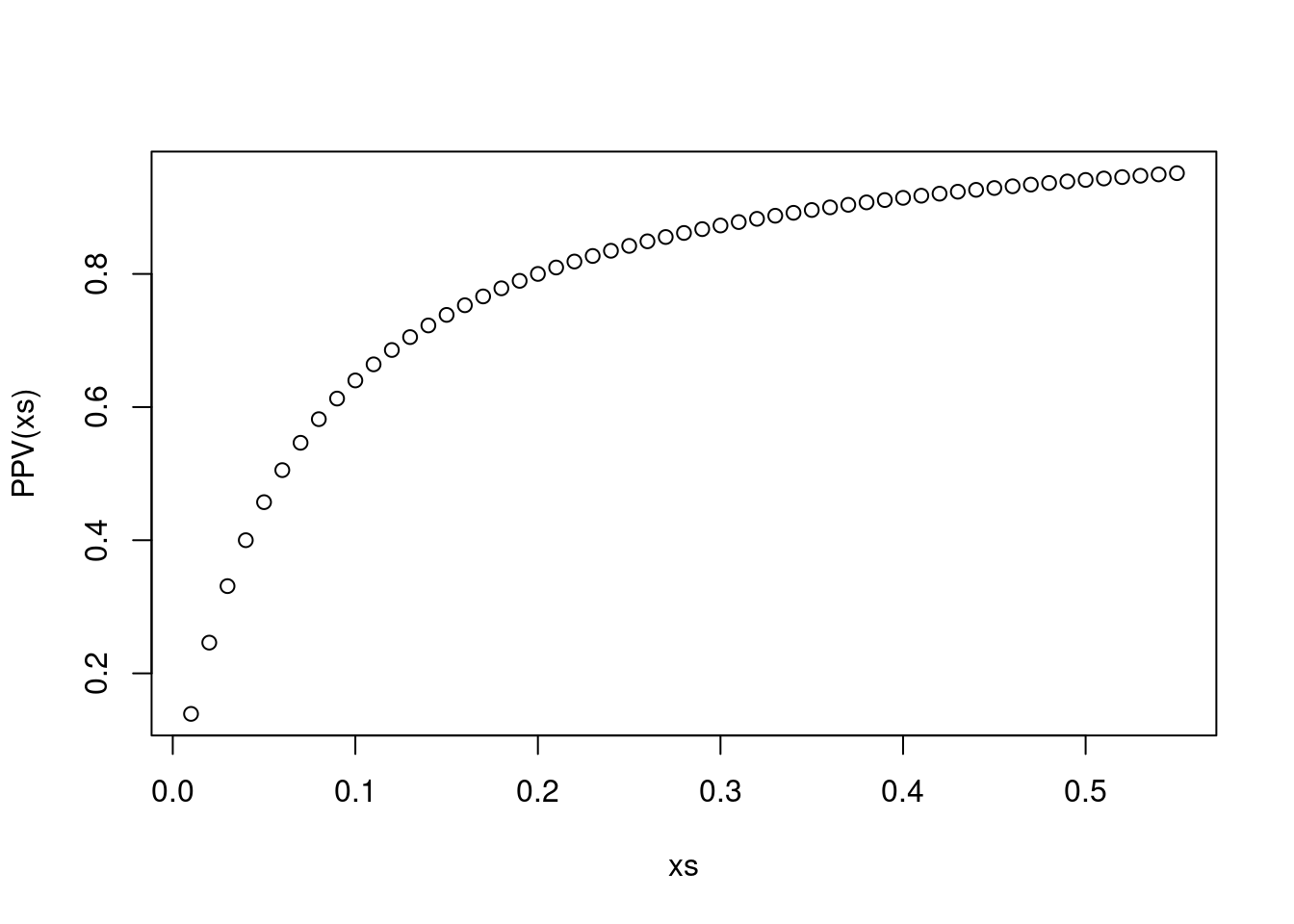

With a power of 0.8 and an alpha of 0.05, the PPV is under 0.8 until you have a true positive prevalence of 0.2. But a lot of hypotheses probably don’t meet that.

To have a PPV of 0.95, we need the following alpha levels:

• prevalence 0.1: p = 0.005
• prevalence 0.05: p = 0.002
• prevalence 0.01: p = 0.0004

How to distinguish true effects from other patterns

The times when this concern is most appropriate are when dealing with studies where the effect size is not so (qualitatively) large and there are conflicting results in different studies. Then it matters a lot whether the null results are being underrepresented in the literature. The question isn’t about whether null hypothesis testing is useful – it is one of a large range of useful tools that can help rule out apparent patterns that are not of real interest. The real question is, how do we create a literature that people will naturally interpret in an appropriate way?