Sampling the right number of controls

In case-control studies, there is a rule of thumb that you only need to sample about three or four times as many controls as cases. The cases are usually the limiting factor, especially when the disease is rare and they are difficult to find, so it makes sense to sample more controls than cases to boost statistical power. But at a certain point, the cost of managing additional controls is greater than the statistical power they add. This is especially true when it is expensive to assess exposure status. So epidemiologists usually stop when they have a ratio of three or four to one.

It’s pretty easy to test this to see if it makes sense. make_ci_plot(risk_un, RD, p_exp) is a function that constructs a sample from a population with unexposed risk risk_un, risk difference RD, and exposure prevalence p_exp. It uses a range of control to case ratios, from 0.5 to 7, and plots the width of the resulting confidence interval.

make_ci_plot(0.2, 0.1, 0.1)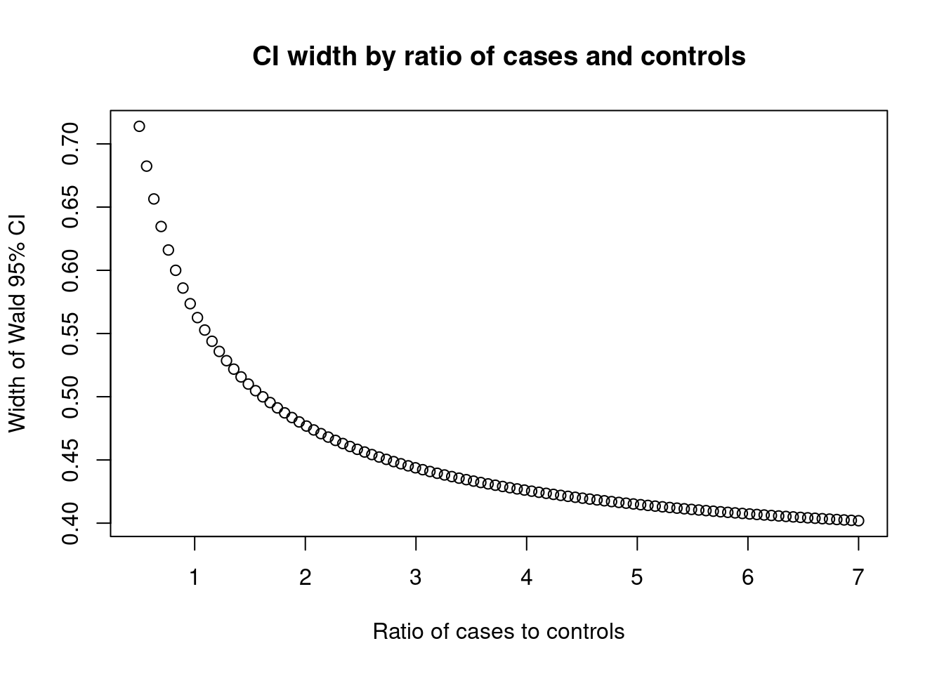

As expected, the confidence interval is very wide with low ratios, but past four there is little to be gained by increasing the control to case ratio.

The characteristics of the source population will affect the confidence interval widths (especially the exposure prevalence), but the shape of the curve is always the same.

make_ci_plot(0.3, 0.01, 0.1)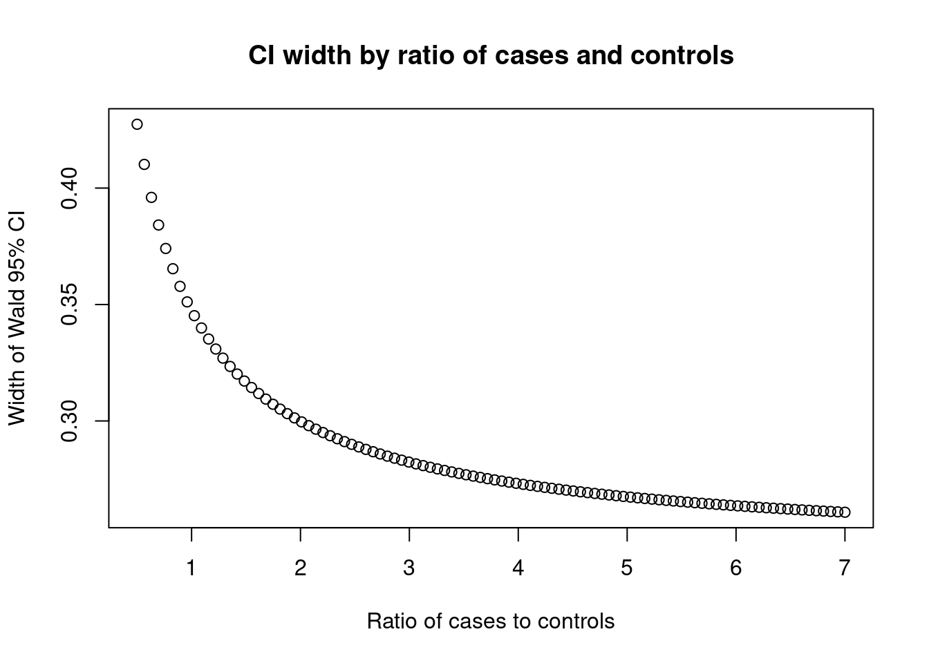

make_ci_plot(0.25, 0.1, 0.01)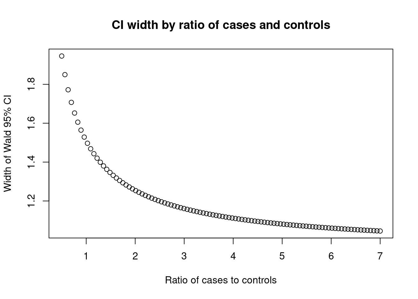

Source code

library(epitools)

# Make 2x2 table given unexposed risk, risk difference, prevalence of
# exposure, and sample size, using case-cohort sampling
get_cells <- function (risk_un, RD, p_exp, n = 10000) {
  risk_exp <- risk_un + RD
  a <- n * risk_exp * p_exp
  b <- n * risk_un * (1 - p_exp)

  c(
    a,
    b,
    (n - a - b) * p_exp,
    (n - a - b) * (1 - p_exp)
  )
}

# calculate the CI width given the 2x2 table
get_ci_width <- function(cells) {
  ests <- as.data.frame(oddsratio.wald(cells)$measure)[2,]
  ests$upper - ests$lower
}

get_widths <- function(samples) {
  lapply(samples, function (x) { get_ci_width(x) })
}

# sample from the controls
make_sample <- function(pop, size) {
  c(pop[1:2], pop[3:4] * size)
}
 
make_samples <- function(pop, sizes) {
  lapply(sizes, function (x) { make_sample(pop, x) })
}

# convert between ratio of controls to cases and
# the amount of controls needed to sample
calc_ratio <- function(size, cells) {
  (sum(cells[3:4]) * size) / sum(cells[1:2]) 
}

calc_size <- function(ratio, cells) {
  ratio * sum(cells[1:2]) / sum(cells[3:4])
}

# set sampling for control-case ratios of 0.5 to 7
get_sizes <- function(cells) {
  seq(calc_size(0.5, cells), calc_size(7, cells), length.out = 100)
}

# sample and plot the results
make_ci_plot <- function(risk_un, rd, p_exp) {
  cells <- get_cells(risk_un, rd, p_exp)
  sizes <- get_sizes(cells)

  plot(
    x = calc_ratio(sizes, cells),
    y = get_widths(make_samples(cells, sizes)),
    xlab = "Ratio of cases to controls",
    ylab = "Width of Wald 95% CI",
    main = "CI width by ratio of cases and controls"
  )
}

Epi Notes

Sampling the right number of controls

Source code